2 Operating Models
The operating models (OMs) are conditioned using the S05 assessment model (see Section 1.2) as a base case.
The S05 assessment model is referred to as the Reference OM.
2.1 Reference Set
The Reference Set OMs are currently designed as a factorial uncertainty grid with two axes of uncertainty:
- Growth: uncertainty in the von Bertalanffy parameters
- Natural mortality: uncertainty in the reference M of the Lorenzen natural mortality curve.
Additional operating models may be added to the Reference OMs - e.g., uncertainty in the steepness parameter of the Beverton-Holt stock recruit relationship.
Each axis is represented at three levels, corresponding to the 25th, 50th, and 75th percentiles of the estimated parameter values. The 50th percentile level for each axis matches the S05 reference assessment, so the combination of the two 50th-percentile levels corresponds to the Reference OM.
This produces a 3 x 3 uncertainty grid with 9 reference operating models.
The von Bertalanffy growth parameters at each percentile level are shown in Table 2.1.
Each level for natural mortality is defined by a reference Lorenzen M value (at reference age 11), which determines the full age-specific M vector via the Lorenzen relationship.
Because this relationship scales with weight-at-age, the resulting M-at-age vector also depends on growth, Table 2.2 shows the vector at the 50th-percentile of the growth parameters (see Table 2.1) only. The vectors for the 25th- and 75th-percentile growth scenarios differ slightly from these values.
| Percentile | \(L_\infty\) | \(K\) | \(t_0\) |
|---|---|---|---|
| 25th | 115.93 | 0.235 | -0.561 |
| 50th (Base Case) | 121.24 | 0.238 | -0.891 |
| 75th | 125.02 | 0.237 | -1.217 |
| Age | 25th | 50th (Base Case) | 75th |
|---|---|---|---|
| 0 | 0.778 | 0.966 | 1.180 |
| 1 | 0.560 | 0.695 | 0.849 |
| 2 | 0.459 | 0.570 | 0.697 |
| 3 | 0.403 | 0.500 | 0.611 |
| 4 | 0.367 | 0.456 | 0.557 |
| 5 | 0.343 | 0.426 | 0.521 |
| 6 | 0.327 | 0.405 | 0.495 |
| 7 | 0.314 | 0.390 | 0.477 |
| 8 | 0.306 | 0.379 | 0.464 |
| 9 | 0.299 | 0.371 | 0.454 |
| 10 | 0.294 | 0.365 | 0.446 |
| 11 | 0.290 | 0.360 | 0.440 |
| 12 | 0.287 | 0.356 | 0.435 |
| 13 | 0.285 | 0.353 | 0.432 |
| 14 | 0.283 | 0.351 | 0.429 |
| 15 | 0.280 | 0.348 | 0.425 |
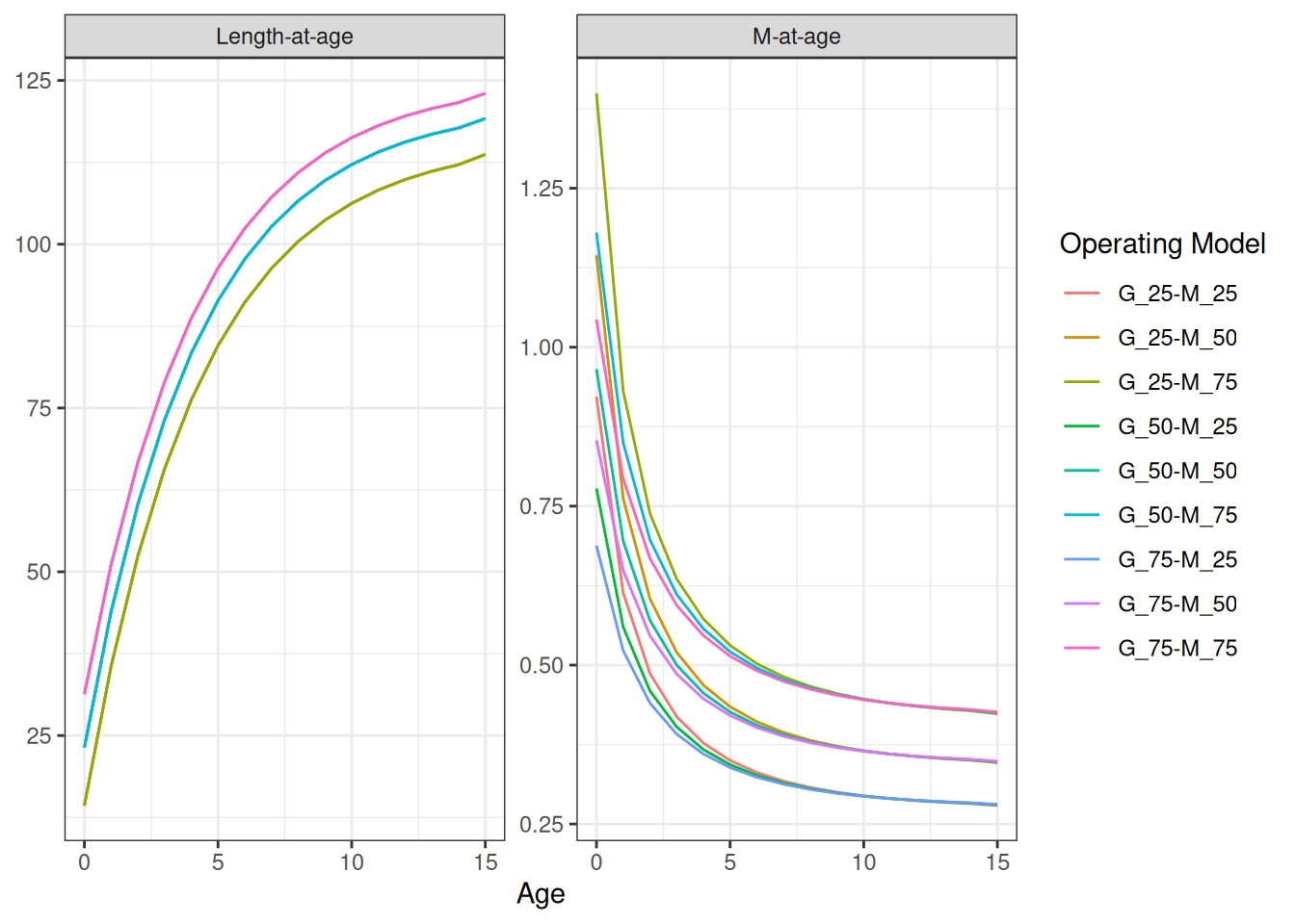
2.1.1 Overview of Reference OMs
Figure 2.1 shows the length- and natural mortality-at-age curves for each of the 9 reference grid OMs.
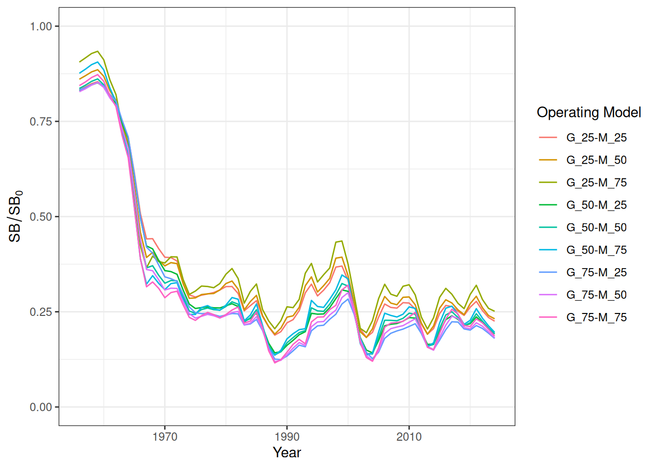
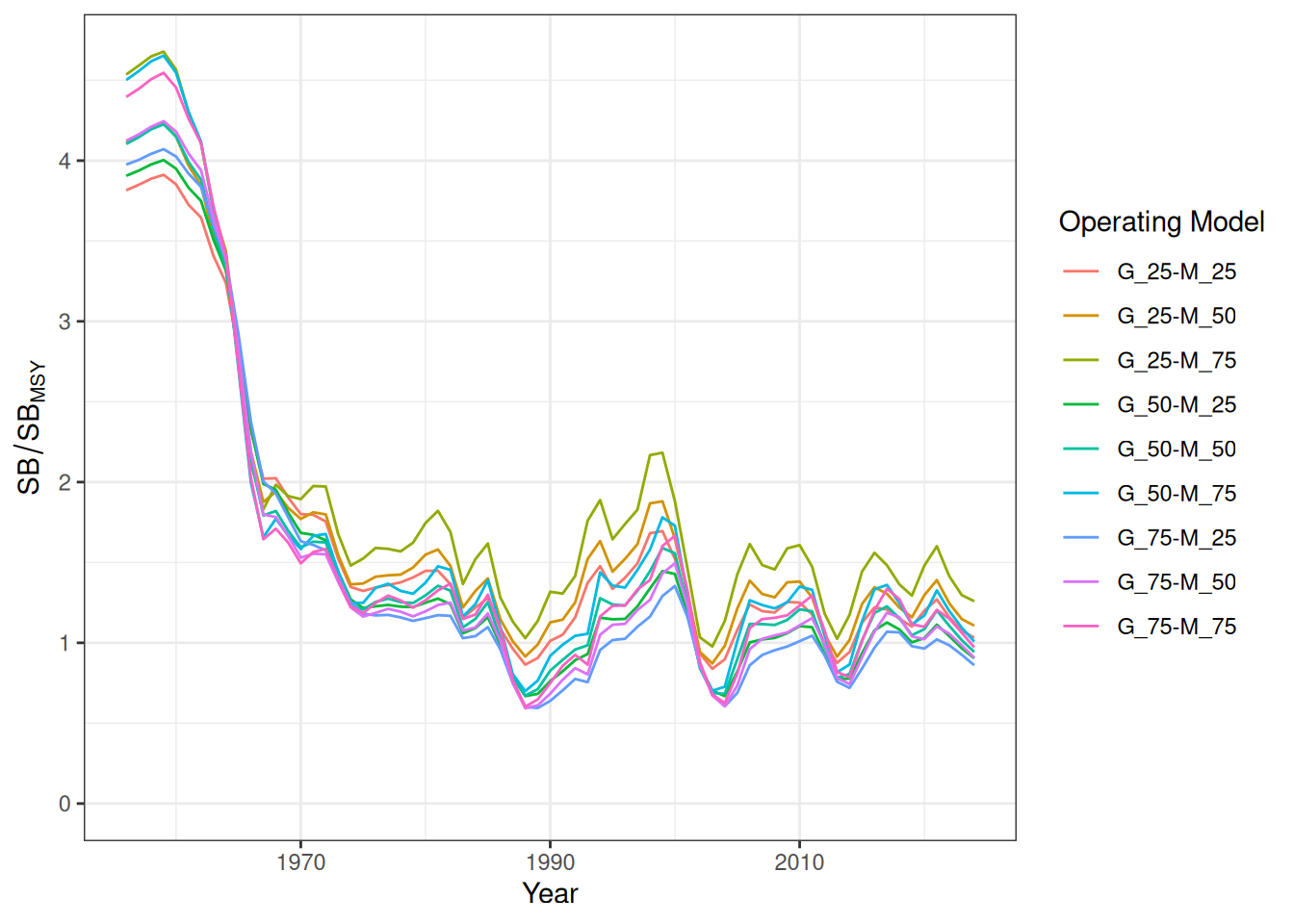
Figure 2.2 shows the historical spawning biomass depletion (\(SB/SB_0\)) trajectory for each of the 9 reference grid OMs, while Figure 2.3 shows the spawning biomass relative to the MSY level.
2.2 Robustness OMs
Robustness OMs have not yet been developed for SALB.
Potential Robustness OMs may include:
- uncertainty in TAC implementation (e.g., overages in TAC)
- impacts of climate change (e.g., time-varying life-history parameters)
- alternative recruitment scenarios.