2  Operating Models

2.1 OM Conditioning

The operating models were based on the recent SALB stock assessment, completed in June 2026 using the Stock Synthesis 3 (SS3) assessment framework (Methot and Wetzel 2013). See the Report of the 2026 ICCAT Albacore Stock Assessment Meeting and the Report of the 2026 ICCAT Albacore Data Preparatory Meeting for full details on the stock assessment.

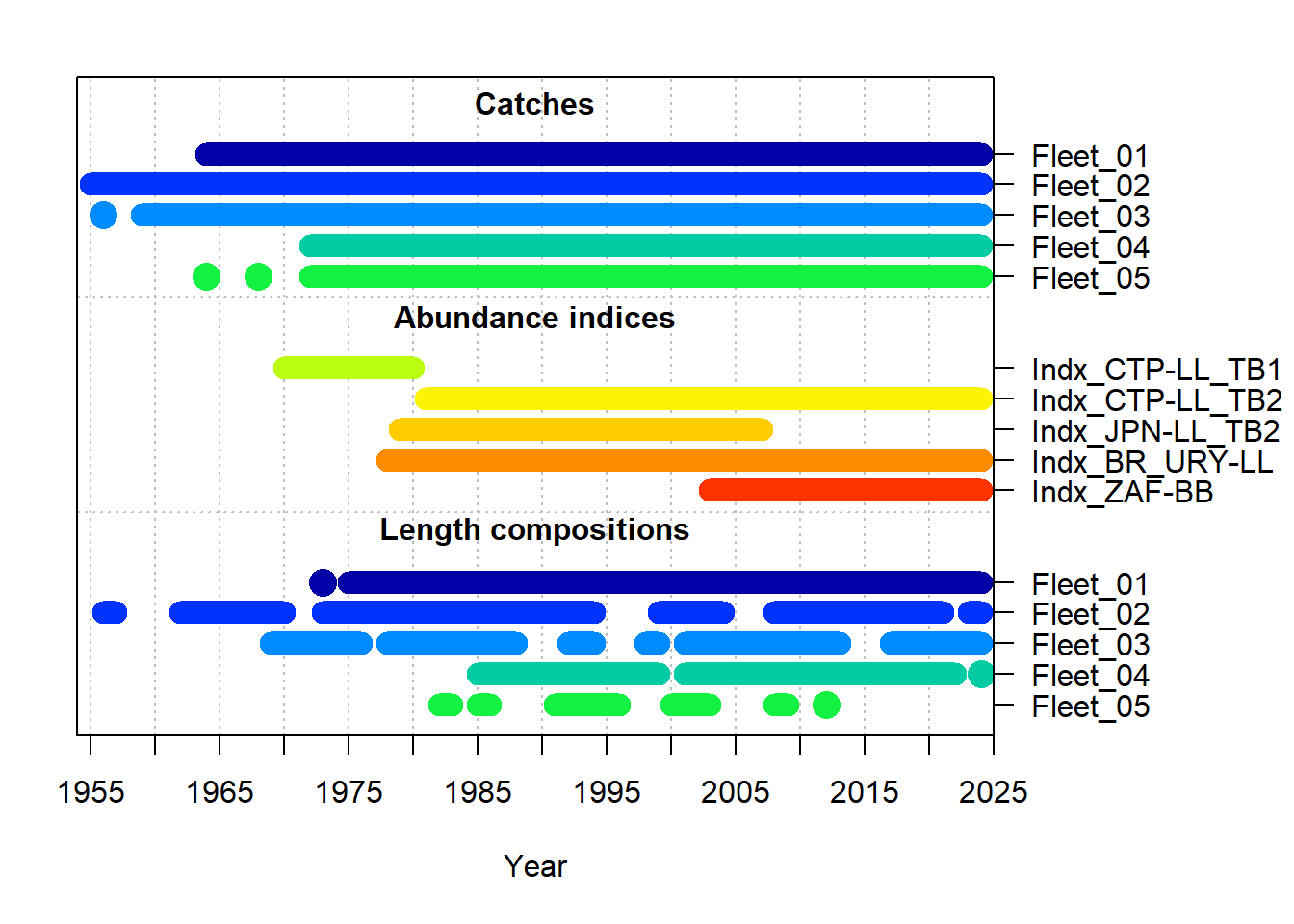
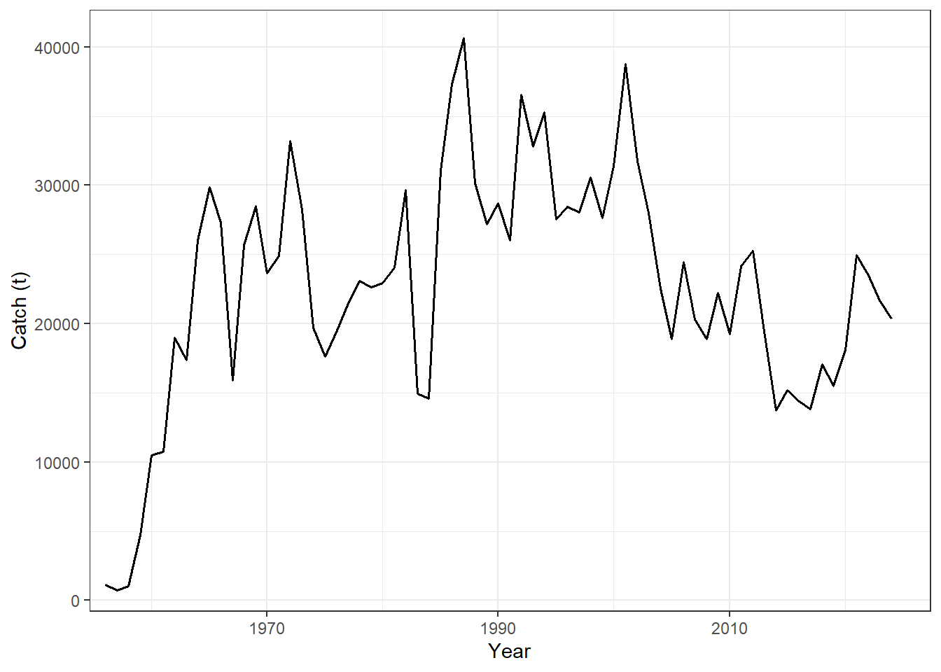
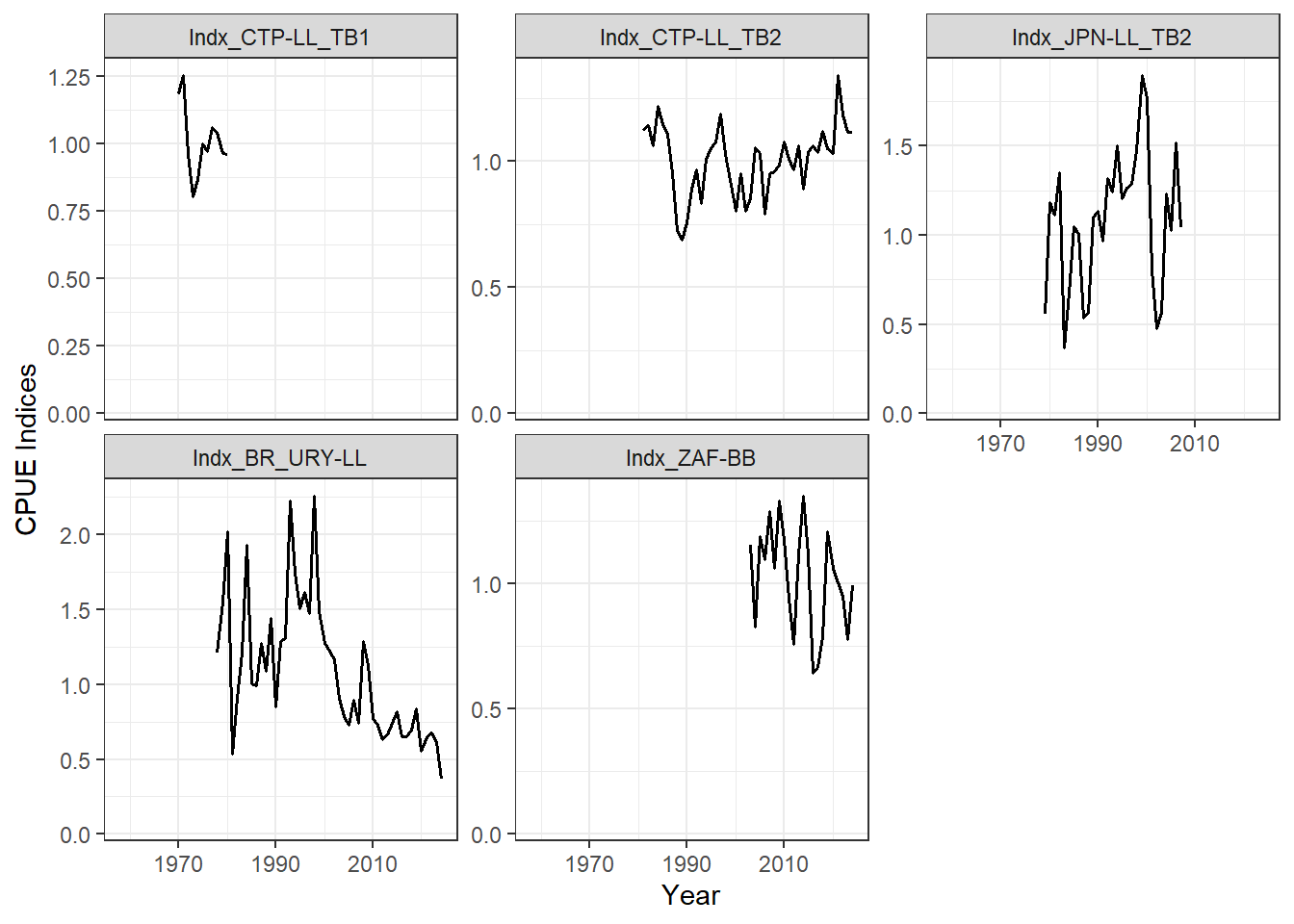
The assessment model integrated total catches, standardized indices of abundance, and length-composition data covering the period 1956 – 2024. Five fishing fleets were defined by aggregating catch and length composition data for fishing fleets with similar properties (Table 2.1; Figure 2.1; Figure 2.2). Five standardized CPUE indices were used in the Base Case assessment (Table 2.2; Figure 2.1; Figure 2.3).

Table 2.1: Fleet structure, data and time periods to be used in the South Atlantic albacore Stock Synthesis model. Adapted from Table 11 in the Data Preparatory Report.

Fleet	Definition (FlagName and Gear Group)	Catch	Size composition data
Fleet 1	Chinese Taipei (LL), Korea (LL)	1964-2024	up to 2024
Fleet 2	Japan (LL), China (LL), EU-Spain (LL), EU-Portugal (LL), USA (LL), Philippines (LL), St Vincent and Grenadines (LL), Vanuatu (LL), Honduras (LL), NEI (LL), Côte D’Ivoire (LL), United Kingdom (LL), Seychelles (LL), UK.Sta Helena (LL), Angola (LL), Senegal (LL), Trinidad and Tobago (LL)	1956-2024	1956-2024
Fleet 3	Brazil (LL, SU), Uruguay (LL), Namibia (LL), Panama (LL), South Africa (LL, UN), Argentina (LL, TW, UN), Belize (LL), Cambodia (LL), Cuba (LL, UN)	1959-2024	1969-2024
Fleet 4	South Africa (BB, HL, PS, RR, SP)	1973-2024	1980-2024
Fleet 5	All others	1961-2024	1961-2024

Table 2.2: CPUE indices and time periods to be used in the South Atlantic albacore Stock Synthesis model. Adapted from Table 11 in the Data Preparatory Report.

Index Name	Definition	Years
Indx_CTP-LL_TB1	Chinese Taipei longline, time block 1	1970-1980
Indx_CTP-LL_TB2	Chinese Taipei longline, time block 2	1981-2024
Indx_JPN-LL_TB2	Japan longline	1979-2017
Indx_BR_URY-LL	Brazil/Uruguay longline	1978-2024
Indx_ZAF-BB	South Africa baitboat	2003-2024

Figure 2.1: Overview of the data used in the 2026 stock assessment.

Figure 2.2: Time series plot of the total catch data used in the 2026 assessment.

Figure 2.3: Time series plot of the five CPUE indices used in the Base Case 2026 assessment.

2.2 Primary Uncertainties

The primary uncertainties identified during the stock assessment process related to the life-history parameters related to growth and natural mortality rate, and the conflicting signals in the indices of abundance that were fit in the assessment (see assessment reports linked above).

2.2.1 Life History Parameters

Following the assessment, growth was modelled with the von Bertalanffy function with parameters \(L_\infty\), \(K\), and \(t_0\) describing the mean asymptotic length, the Brody growth coefficient, and the theoretical age where mean length is 0 respectively. Natural mortality (M) was modelled with the Lorenzen function which assumes decreasing natural mortality as fish increase in size (Lorenzen et al. 2022). The stock-recruitment relationship modelled with the Beverton-Holt equation, parameterized with steepness (h) fixed at 0.75. Maturity was specified as an at-age schedule with fish reaching 50% maturity at age 5 years and full maturity at 6 years. See Table 5 in the Data Preparatory Report for a full list of the life-history parameters used in the model.

The von Bertalanffy parameters and the natural mortality rate were identified as the primary life-history uncertainties. To account for these uncertainties, a factorial uncertainty grid was developed spanning the two axes of uncertainty (Growth and Natural Mortality), each with three levels corresponding to the 25th, 50th, and 75th percentiles of the estimated distributions for these parameters (Table 2.3). The 50th percentile level for each axis matches the Base Case stock assessment model.

Table 2.3: von Bertalanffy growth parameters and reference natural mortality (\(M\)) at each level of the uncertainty grid.

Percentile	\(L_\infty\)	\(K\)	\(t_0\)	\(M\)
25th	115.93	0.235	-0.561	0.29
50th (Base Case)	121.24	0.238	-0.891	0.36
75th	125.02	0.237	-1.217	0.44

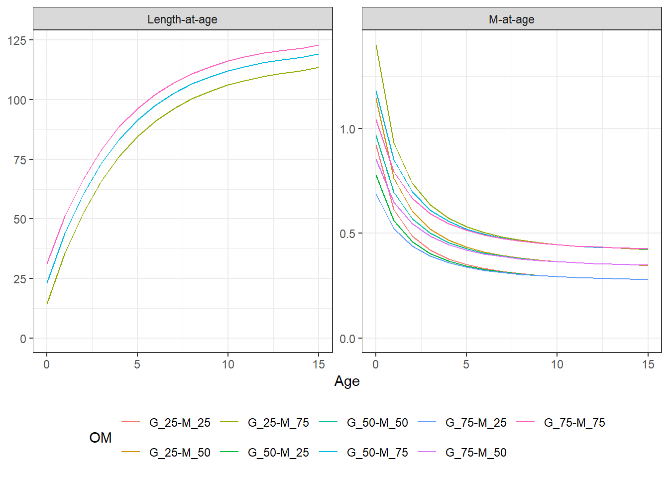
The three levels for each axis produces a 3 x 3 uncertainty grid with 9 variations (Table 2.4). Figure 2.4 shows the length- and natural mortality-at-age curves for each of the 9 combination of parameters in the uncertainty grid.

Table 2.4: The uncertainty grid spanning two axes of uncertainty, each with three levels.

#	OM	Growth	Natural Mortality
1	G_25-M_25	25th	25th
2	G_25-M_50	25th	50th
3	G_25-M_75	25th	75th
4	G_50-M_25	50th	25th
5	G_50-M_50	50th	50th
6	G_50-M_75	50th	75th
7	G_75-M_25	75th	25th
8	G_75-M_50	75th	50th
9	G_75-M_75	75th	75th

Figure 2.4: The mean length-at-age and natural mortality-at-age schedules for each level in the life-history uncertainty grid.

2.2.2 Indices of Abudance

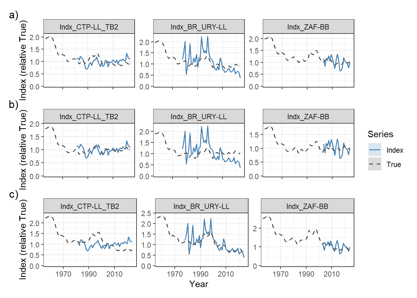
The primary uncertainty in the indices of abundance used in the stock assessment related to two of the three indices that continue through to the terminal year having conflicting trends in recent years: the Chinese Taipei index has an increasing trend in recent years, and the Brazil-Uruguay index has a declining trend (Figure 2.5).

Figure 2.5: The three indices of abundance that continue through to the terminal year (blue solid lines): Chinese Taipei (Indx_CTP-LL_TB2), Brazil Uruguay (Indx_BR_URL-LL), and South Africa bait boat (Index_ZAF-BB) plotted together with the corresponding population biomass trend as described in the central OM (50th percentile for both axes) for a) the Reference models where all three indices were fit in the assessment model), b) R1 where the Brazil Uruguay index was excluded from the likelihood, and c) R2 where the Chinese Taipei index was excluded from the likelihood (black dashed line).

2.3 Reference and Robustness OMs

A set of nine Reference OMs were conditioned using the factorial uncertainty grid (Table 2.3) and following the stock assessment methodology of including all indices in the conditioning process (Figure 2.5).

Two additional Robustness sets of OMs were developed to span the uncertainty in the indices of abundance. The robustness models used the same factorial uncertainty grid as the Reference OMs, but varied in how the indices were treated in the SS3 conditioning model.

The first robustness set, R1, excluded the Brazilian–Uruguay index with the declining trend from the likelihood, while the second robustness set, R2, excluded the Chinese Taipei index (Figure 2.5).

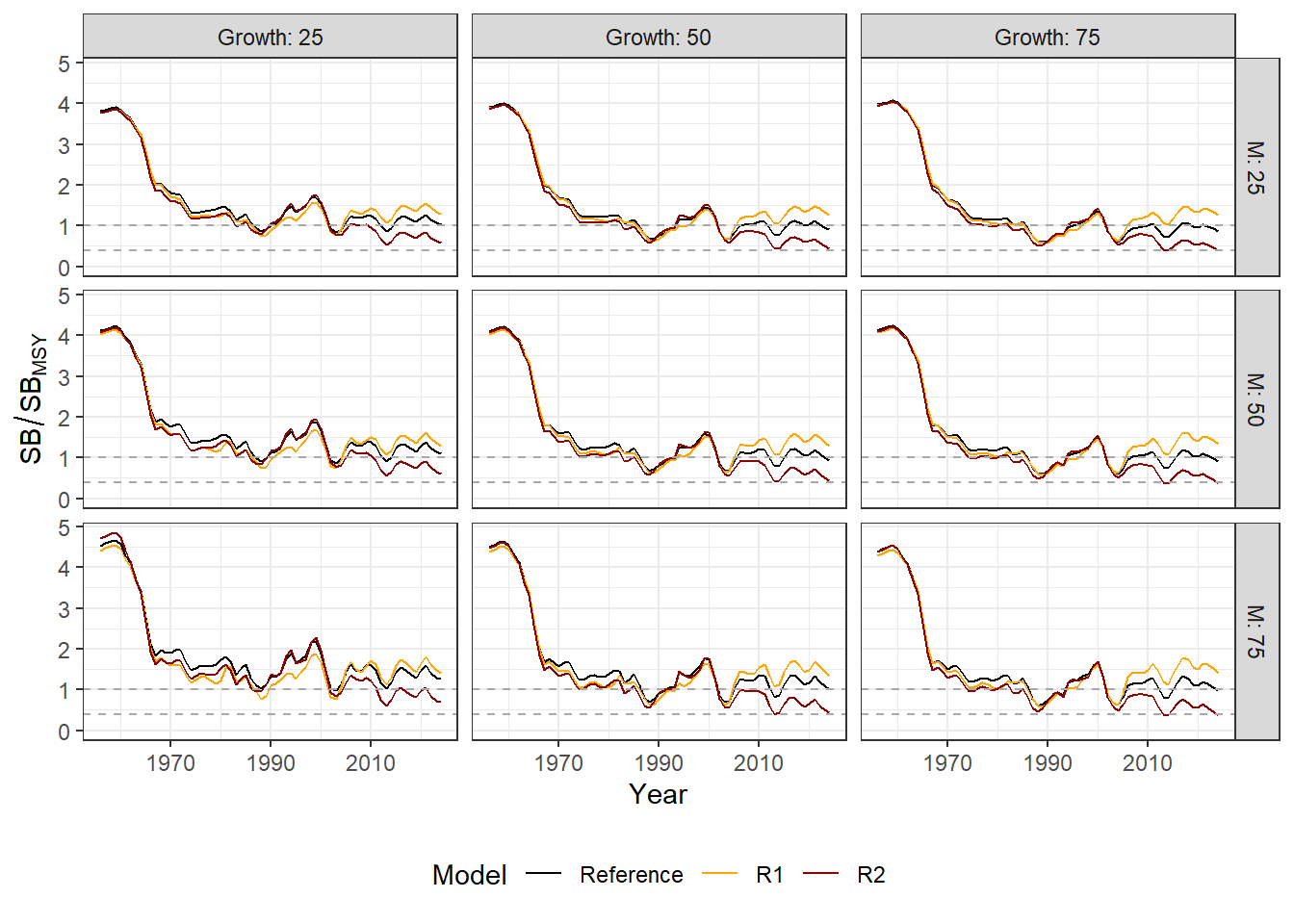
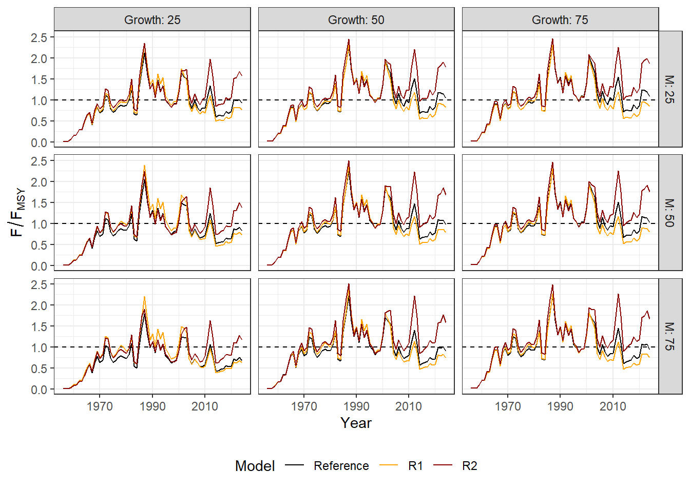
The estimated spawning biomass from the nine Reference OMs was distributed around \(SB_{\text{MSY}}\), with \(SB/SB_{\text{MSY}}\) ranging from 0.86 to 1.26 and \(F/F_{\text{MSY}}\) ranging from 0.68 to 1.08, with the more pessimistic estimates of stock status corresponding with the higher Growth and lower Natural Mortality percentiles (Table 2.5; Figure 2.6; Figure 2.7).

The OMs in the R1 Robustness set had consistently higher estimates of \(SB/SB_{\text{MSY}}\) and lower values of \(F/F_{\text{MSY}}\) for each OM compared to the Reference Set, ranging from 1.26 to 1.41 and 0.63 to 0.84 respectively (Table 2.5; Figure 2.6; Figure 2.7).

The R2 Robustness Set resulted in more pessimistic estimates of stock status compared to the Reference Set, with \(SB/SB_{\text{MSY}}\) and \(F/F_{\text{MSY}}\) ranging from 0.38 to 0.69 and 1.17 to 1.86 respectively (Table 2.5; Figure 2.6; Figure 2.7).

The MSY-based reference points (\(F_{\text{MSY}}\), \(SB_{\text{MSY}}\), and \(MSY\)) estimated for each OM in the Reference, R1, and R2 sets are reported in Table 2.6.

\(F_{\text{MSY}}\) was most sensitive to the Natural Mortality axis, ranging from 0.28 to 1.58 across the uncertainty grid and OM sets, increasing with higher Natural Mortality percentiles and decreasing with higher Growth percentiles.

\(SB_{\text{MSY}}\) was also primarily driven by the Natural Mortality axis, ranging from 14,732 t to 37,721 t, with only a modest reduction across the Growth axis.

In contrast, estimated \(MSY\) was comparatively stable across the uncertainty grid and among the three OM sets, ranging from 23,120 t to 25,876 t, reflecting the offsetting effects of the Growth and Natural Mortality uncertainty axes on stock productivity.

Table 2.5: Summary of the estimated stock status (\(SB/SB_{\text{MSY}}\) and \(F/F_{\text{MSY}}\)) in the terminal year (2024) for the nine operating models from the Growth and Natural Mortality uncertainty grid for the Reference Set and the R1 and R2 Robustness Sets.

	Reference		R1		R2
Growth/Natural Mortality	SB/SBMSY	F/FMSY	SB/SBMSY	F/FMSY	SB/SBMSY	F/FMSY
G_25-M_25	1.03	0.92	1.28	0.77	0.57	1.57
G_25-M_50	1.11	0.82	1.30	0.72	0.61	1.38
G_25-M_75	1.26	0.68	1.41	0.63	0.69	1.17
G_50-M_25	0.90	1.04	1.26	0.83	0.44	1.78
G_50-M_50	0.94	0.97	1.29	0.79	0.43	1.69
G_50-M_75	1.01	0.90	1.34	0.74	0.43	1.59
G_75-M_25	0.86	1.08	1.26	0.84	0.38	1.86
G_75-M_50	0.91	1.02	1.33	0.80	0.38	1.76
G_75-M_75	0.97	0.94	1.41	0.75	0.38	1.67

Figure 2.6: Historical spawning biomass relative to MSY level (\(SB/SB_{\text{MSY}}\)), by operating model for the two Robustness OM sets (R1 and R2). The results from the Reference Set OMs are included for comparison.

Figure 2.7: Historical fishing mortality relative to FMSY level (\(F/F_{\text{MSY}}\)), by operating model for the two Robustness OM sets (R1 and R2). The results from the Reference Set OMs are included for comparison.

Table 2.6: The MSY reference points for the nine operating models from the Growth and Natural Mortality uncertainty grid for the Reference Set and the R1 and R2 Robustness Sets.

	Reference			R1			R2
Growth/Natural Mortality	FMSY	SBMSY	MSY	FMSY	SBMSY	MSY	FMSY	SBMSY	MSY
G_25-M_25	0.47	36,507	24,163	0.45	37,651	24,833	0.51	34,543	23,120
G_25-M_50	0.76	25,047	24,677	0.74	25,558	25,151	0.88	23,618	23,486
G_25-M_75	1.32	17,418	25,579	1.32	17,529	25,748	1.58	16,189	23,961
G_50-M_25	0.32	36,216	23,966	0.31	37,721	24,853	0.33	34,799	23,197
G_50-M_50	0.42	24,274	24,333	0.41	25,260	25,252	0.44	23,322	23,520
G_50-M_75	0.58	16,222	24,756	0.56	16,845	25,675	0.63	15,511	23,767
G_75-M_25	0.28	35,423	23,973	0.28	36,925	24,905	0.28	34,334	23,354
G_75-M_50	0.33	23,292	24,337	0.33	24,327	25,376	0.34	22,604	23,687
G_75-M_75	0.41	15,219	24,728	0.40	15,925	25,876	0.43	14,732	23,945