| Index | SD (log-scale) | Lag-1 AC | Last historical year |
|---|---|---|---|
| Indx_CTP-LL_TB2 | 0.197 | 0.795 | 2024 |
| Indx_BR_URY-LL | 0.332 | 0.396 | 2024 |
| Indx_ZAF-BB | 0.187 | 0.186 | 2024 |
5 Forward Projections
This chapter describes the assumptions and settings for the projection years.
Each operating model has 100 independent simulations.
5.1 Management Cycle and Data Lag
The MSE assumed that the first TAC generated by the CMPs will be set in 2028, with a 3-year management cycle and and a 2-year data lag .
This means that the TAC that will be implemented for the 2028 fishing year will be calculated in 2027 using data up to 2025, and then from there the TAC is updated every 3 years (Table 5.1).
| Implementation Year | Calculation Year | Management Year? | TAC decision | DataYear used |
|---|---|---|---|---|
| 2028 | 2027 | Yes | Calculated in 2027, implemented 2028 | 2025 |
| 2029 | 2028 | No | Carries forward 2028’s TAC | — |
| 2030 | 2029 | No | Carries forward 2028’s TAC | — |
| 2031 | 2030 | Yes | Calculated in 2030, implemented 2031 | 2028 |
| 2032 | 2031 | No | Carries forward 2031’s TAC | — |
| 2033 | 2032 | No | Carries forward 2031’s TAC | — |
| 2034 | 2033 | Yes | Calculated in 2033, implemented 2034 | 2031 |
5.2 Initial Projection Years
Following the stock assessment, the OMs have a historical period spanning from 1956 to 2024. Given that the TAC advice generated by the CMPs will be implemented in 2028, the first 3 years of the projection period (2025, 2026, 2027) are, in effect, an extension of the historical period rather than years managed by the CMPs.
Where real catch data (and, for the indices used by index-based CMPs, real CPUE data) become available for these years, they will be used directly in the OM. Where data are not yet available, fleet-specific catches for these years will instead be simulated by resampling from the mean and standard deviation of each fleet’s catches over the preceding four years.
This is necessary because the population dynamics model needs a catch value for every year in order to project the population forward in time. Additionally, the CMPs require a complete data stream up to the data-lag year in order to calculate the first TAC.
As shown in Table 5.1, the 2028 TAC is calculated in 2027 using data up to 2025. Because the historical period ends in 2024, 2025 falls within the projection period and will not yet be observed at the time the MSE was run. For now, the simulated 2025 catch and CPUE index values will be used to calculate the 2028 TAC. If real 2025 data become available, these can replace the simulated values without requiring any change to the underlying MSE framework.
5.3 Recruitment Deviations
Annual recruitment deviations are generated as autocorrelated, bias-corrected log-normal deviates around the stock-recruit relationship. For a given simulation, the (log-scale) deviation in year \(y\) is calculated as:
\[ \varepsilon_y \sim \text{TruncNormal}(\mu, \sigma_R,\ \pm 3\sigma_R) \]
\[ x_y = \rho\, x_{y-1} + \varepsilon_y \sqrt{1-\rho^2} \]
\[ \text{RecDev}_y = \exp(x_y) \]
where \(\sigma_R\) is the recruitment deviation standard deviation, \(\rho\) is the lag-1 autocorrelation, and \(\mu = -0.5\sigma_R^2(1-\rho)/\sqrt{1-\rho^2}\) is a bias-correction term so that \(E[\text{RecDev}_y] = 1\) on the natural scale. Deviations are truncated at \(\pm 3\sigma_R\) (on the log scale) to avoid unrealistic extremes.
5.4 Observation Error for Simulated Data
The data used by the CMPs (fleet-specific catches and standardised CPUE indices) are simulated from the true OM-generated values with multiplicative observation error.
For catch, the observation error is conditioned on the historical fit between the OM’s simulated catch and the actual reported historical catch. In practice, the assessment model is fit to the catch data essentially exactly, so the catch data provided to the CMPs exactly matches the catches in the OM.
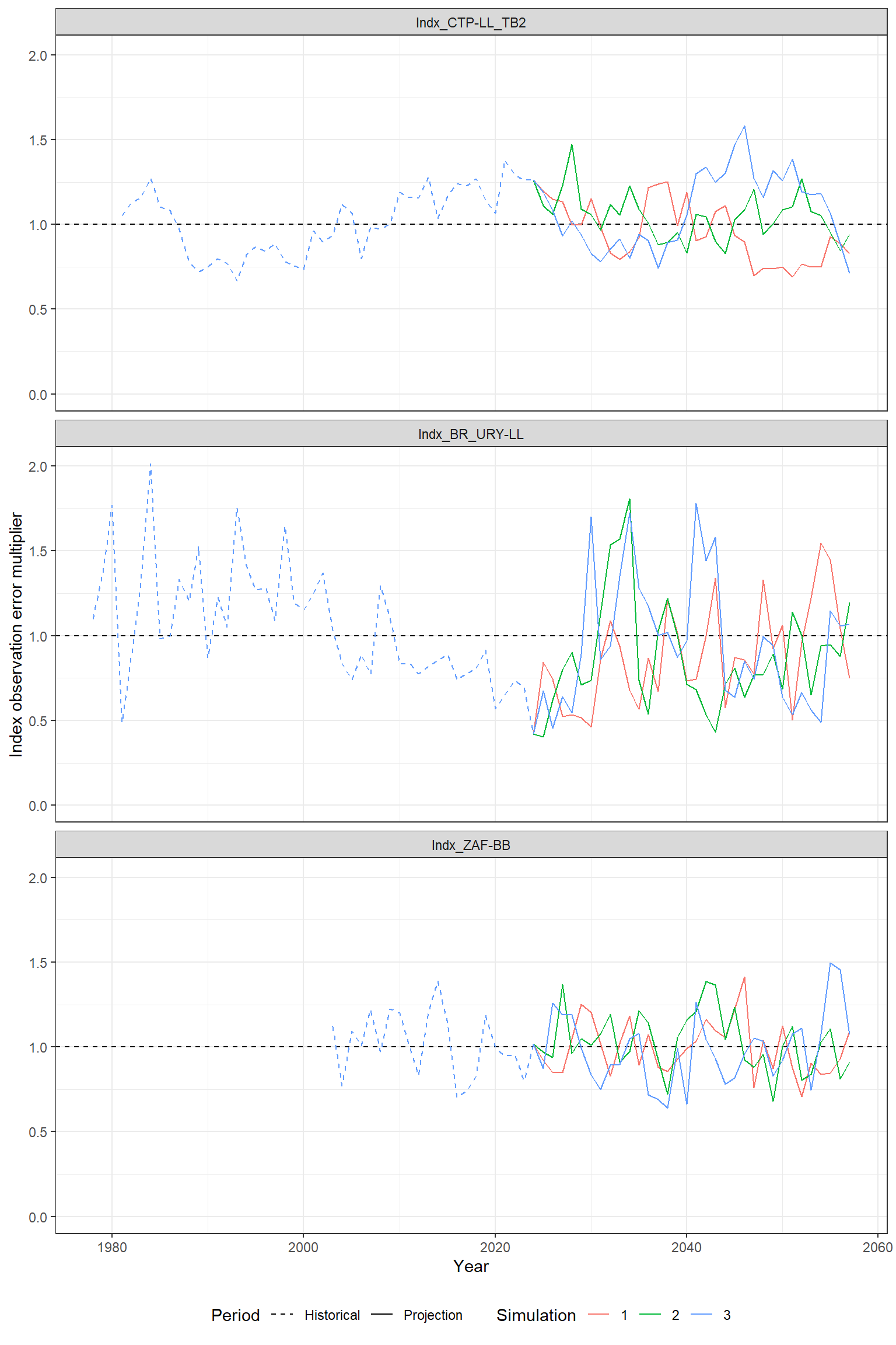
For the CPUE indices, the same historical-conditioning approach is used, but with a lag-1 autocorrelation additionally estimated from the residuals between the observed and simulated index. Index observation error therefore follows the same truncated, autocorrelated log-normal process described above for recruitment deviations, continuing on from the last estimated historical residual.
Table 5.2 shows the fitted SD and lag-1 autocorrelation for each index that is available in the terminal year. All indices are assumed to scale proportionally with true abundance (i.e. no hyperstability/hyperdepletion).
These values are specific to the Reference OM shown here as an example. The conditioned SD and autocorrelation will vary across the full set of Reference and Robustness OMs, since each is conditioned on its own historical fit.
Figure 5.1 shows example realisations of the index observation error multiplier for three simulations, spanning the historical and projection periods, again for the Reference OM only.
It illustrates that the autocorrelated observation error applied in the projections has the same statistical properties as estimated from the historical period.
Historical indices that are no longer produced are excluded, since these will not be generated or used in the projection period.