7 Candidate Management Procedures
Within the MSE framework, each candidate management procedure (CMP) is applied to the historical data simulated by each operating model and then used to set management advice at each management cycle throughout the projection period.
The performance of each CMP is compared across the Reference and Robustness OMs (see Chapter 3 and Chapter 4) using the performance metrics described in Chapter 6.
Four general categories of CMPs have currently been developed. Within each category, several variants have also been developed and tuned, spanning a range from more conservative to more aggressive settings of that category’s tuning parameter.
Note
These CMPs are preliminary, intended to test the MSE framework, and remain subject to further development and refinement by the SALB MSE Technical Team.
7.1 Constant Effort
The Constant Effort CMPs have been developed as a reference method, to evaluate how the stock is expected to perform under a simple, non-reactive fishing strategy, providing a benchmark against which the reactive CMPs below can be compared.
Fishing effort is held fixed at a chosen fraction of the most recent historical effort level for the whole projection period. Because of the assumption of stationary catchability (\(q\)), these fixed effort CMPs correspond to a constant fishing mortality in the projection years.
7.2 Index Rate
The Index Rate CMPs aim to keep a constant exploitation rate throughout the projection years.
Data used: the (equal-weighted) mean of the three abundance indices still being reported, and catch data, although only the catch data from last two historical years are used (see below).
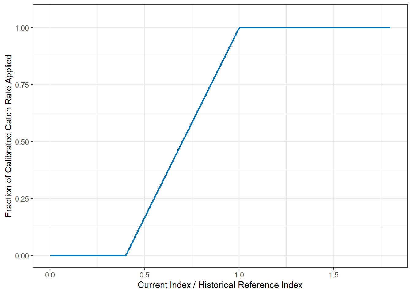
How it works: a catch rate is calibrated once, from the last two years of the historical period, and held fixed for the rest of the projection. That fixed rate is scaled by the tuning parameter, then scaled again by a ramped response to how the current abundance index compares with a historical reference level (2007 – 2010; Figure 7.1):
\[ \hat{r} = \frac{\bar{C}_{\text{hist}}}{\bar{I}_{\text{hist}}}, \qquad C_{\text{limit}} = \hat{r} \times m \times I_{\text{cur}} \times \theta\!\left(\frac{I_{\text{cur}}}{I_{\text{ref}}}\right) \]
where \(\bar{C}_{\text{hist}}\) and \(\bar{I}_{\text{hist}}\) are the average catch and index over the last two years of the historical period, \(I_{\text{cur}}\) is the current abundance index, \(m\) is the tuning parameter, and \(\theta(x)\) ramps the response from zero at a defined lower limit up to a full response once the index reaches a healthier reference level:
\[ \theta(x) = \begin{cases} 0 & x \le x_L \\[4pt] \dfrac{x - x_L}{x_U - x_L} & x_L < x < x_U \\[4pt] 1 & x \ge x_U \end{cases} \]
The resulting catch limit is also capped in how much it can change from one management cycle to the next (up to 40%, in either direction).
7.3 Index Target
The Index Target CMPs move the catch limit directly in proportion to how far the current abundance index sits from a historical reference level.
Data used: the same three abundance indices, compared against the same historical reference period (2007 – 2010) used by Index Rate.
How it works: the catch limit moves up or down each management cycle in direct proportion to how the current abundance index compares with that historical reference level, and that change is capped (up to 40% down, 20% up) before the tuning parameter and a throttle are applied on top:
\[ \frac{C_{\text{limit}}}{C_{\text{prev}}} = \frac{I_{\text{cur}}}{I_{\text{target}}} \times m \times \theta\!\left(\frac{I_{\text{cur}}}{I_{\text{target}}}\right) \]
using the same ramped response \(\theta\) introduced under Index Rate above, but here with its lower limit and upper reference level set to the same value; i.e., rather than ramping, the response is a hard cutoff, giving the full proportional response above that index level and none at or below it.
7.4 Stepped Index-Based (MCC)
Based on the Mostly Constant Catch (MCC) design ICCAT adopted for North Atlantic swordfish.
Data used: the three abundance indices, combined into a single index series. Each index’s contribution to that combined series is weighted by its own reported precision (inverse variance, i.e. \(1/CV^2\)).
How it works: the combined index from the most recent year is compared with the average over the same 2007 – 2010 historical reference period used by Index Rate and Index Target. That ratio determines which of several pre-agreed bins applies (Table 7.1), each with its own multiplier on a baseline catch level: the last historical year’s total landings, scaled by the tuning parameter.
\[ I_{\text{rat}} = \frac{\bar{I}_{\text{cur}}}{\bar{I}_{\text{hist}}}, \qquad \text{TAC}_{\text{base}} = C_{\text{LHY}} \times m, \qquad C_{\text{limit}} = \text{TAC}_{\text{base}} \times s(I_{\text{rat}}) \]
where \(\bar{I}_{\text{cur}}\) is the combined index averaged over the most recent year, \(\bar{I}_{\text{hist}}\) is its average over the historical reference period, \(C_{\text{LHY}}\) is the last historical year’s total landings, \(m\) is the tuning parameter, and \(s(\cdot)\) is the step function in Table 7.1.
| Combined Index / Historical Base (\(I_{\text{rat}}\)) | TACbase multiplier |
|---|---|
| < 0.65 | 0.30 |
| 0.65 – 0.80 | 0.75 |
| 0.80 – 1.20 | 1.00 |
| 1.20 – 1.30 | 1.20 |
| 1.30 – 1.40 | 1.30 |
| 1.40 – 1.50 | 1.40 |
| 1.50 – 1.60 | 1.50 |
| 1.60 – 1.70 | 1.60 |
| >= 1.70 | 1.70 |
7.5 SPiCT
SPiCT (Stochastic surplus Production model in Continuous-Time) is a state-space surplus production model.
Data used: the total catch series and the three indices, fit inside the model (Schaefer production curve) that is re-run at every management cycle using the latest data. Each index’s assumed precision in the fit is set from its own reported CV, rescaled relative to the mean CV across the indices currently in use, so an index reported as proportionally less precise than the others is down-weighted in the fit.
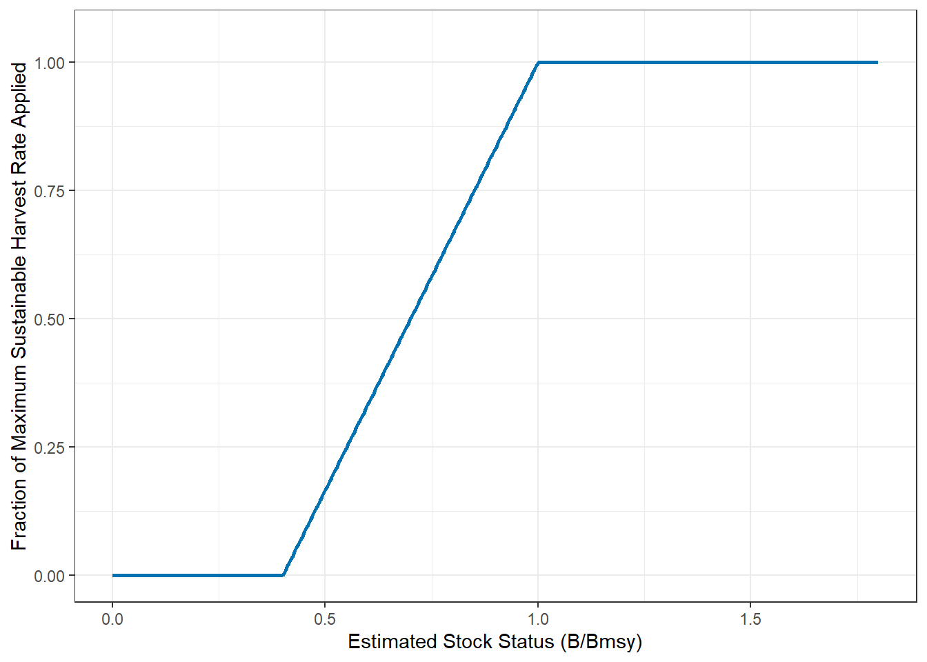
How it works: the fitted model’s estimate of current stock status relative to \(B_{\text{MSY}}\) is rescaled by the tuning parameter and passed through the same style of ramped response used by Index Rate above (Figure 7.2), giving a fraction of \(F_{\text{MSY}}\) to apply as the harvest rate. That rate is applied to the model’s estimate of current biomass, itself also rescaled by the tuning parameter, to set the catch limit:
\[ \widehat{B/B}_{\text{MSY}} = \frac{B_{\text{est}}}{B_{\text{MSY,est}}} \times s, \qquad C_{\text{limit}} = \, F_{\text{MSY,est}} \times \theta\!\left(\widehat{B/B}_{\text{MSY}}\right) \times B_{\text{est}} \times s \]
where \(B_{\text{est}}\), \(B_{\text{MSY,est}}\), and \(F_{\text{MSY,est}}\) are all estimated by the model refit that cycle, \(m\) is the tuning parameter, and \(\theta\) is the ramped response introduced under Index Rate above, here with its control points set at 0.4 (limit) and 1 (full response).
The resulting catch limit is capped in how much it can change from one management cycle to the next: up to 30% down, 50% up. If the model fails to fit or converge in a given cycle, the catch limit is held at its previous value.