3 Reference Operating Models

The Reference Set OMs are currently designed as a factorial uncertainty grid with the two axes of uncertainty (Growth & Natural Mortality) developed during the 2026 Stock Assessment (see Chapter 2).

The Growth and Natural Mortality axes were both represented with three levels, corresponding to the 25th, 50th, and 75th percentiles of the estimated parameter distributions. The 50th percentile level for each axis matches the Base Case stock assessment model (S05).
The OM imported from this model is referred to as the Reference OM.

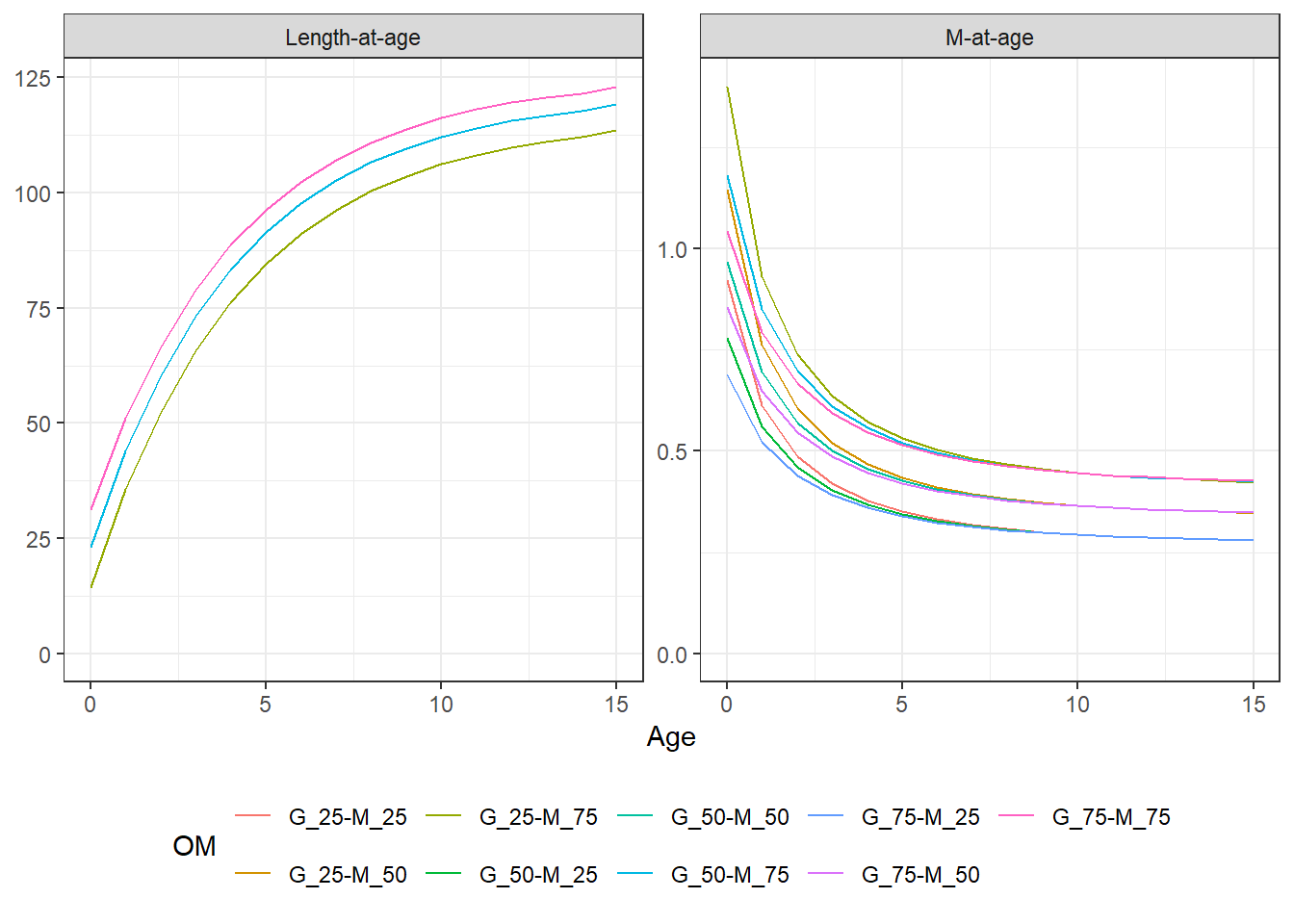
The three levels for each axis produces a 3 x 3 uncertainty grid with 9 reference operating models (Table 3.1). The von Bertalanffy growth parameters and the reference Lorenzen M value (at reference age 11) at each percentile level are shown in Table 3.2.

Figure 3.1 shows the length- and natural mortality-at-age curves for each of the 9 reference grid OMs.

Table 3.1: Grid of nine reference operating models (OMs) spanning two axes of uncertainty, each with three levels.

#	OM	Growth	Natural Mortality
1	G_25-M_25	25th	25th
2	G_25-M_50	25th	50th
3	G_25-M_75	25th	75th
4	G_50-M_25	50th	25th
5	G_50-M_50	50th	50th
6	G_50-M_75	50th	75th
7	G_75-M_25	75th	25th
8	G_75-M_50	75th	50th
9	G_75-M_75	75th	75th

Table 3.2: von Bertalanffy growth parameters and reference natural mortality (\(M\)) at each level of the OM uncertainty grid.

Percentile	\(L_\infty\)	\(K\)	\(t_0\)	\(M\)
25th	115.93	0.235	-0.561	0.29
50th (Base Case)	121.24	0.238	-0.891	0.36
75th	125.02	0.237	-1.217	0.44

Figure 3.1: Length-at-age and natural mortality-at-age, by operating model.

3.1 Overview of Population Dynamics

Each operating model was imported from the maximum likelihood estimates (MLE) of the corresponding SS3 run, so within each OM the historical population dynamics are identical across simulations.

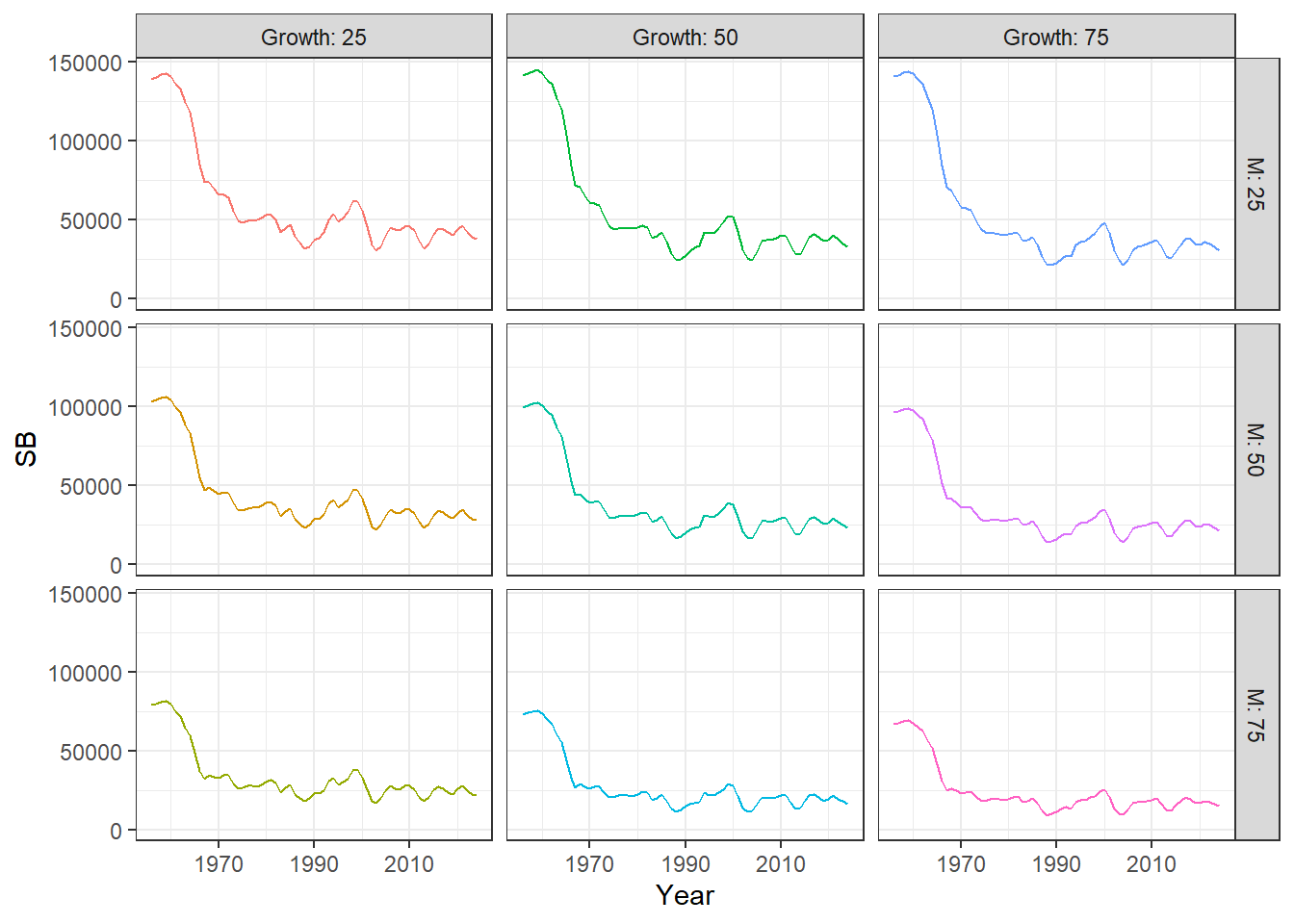
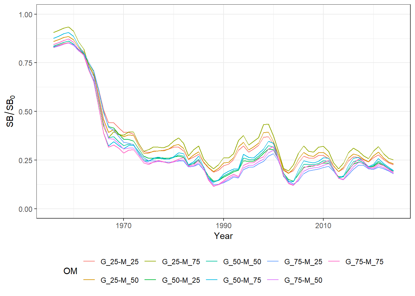
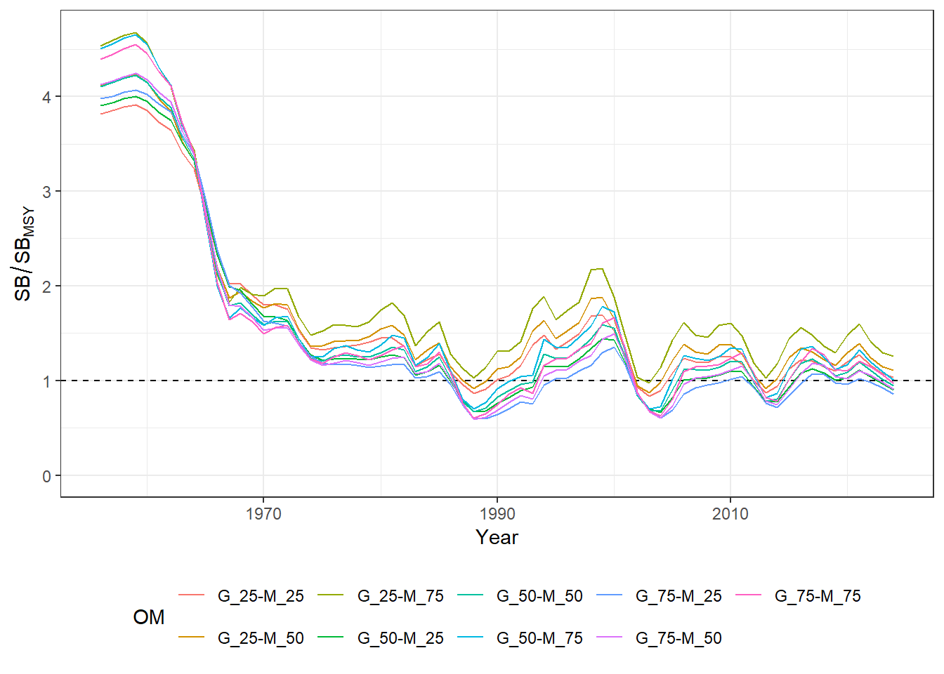
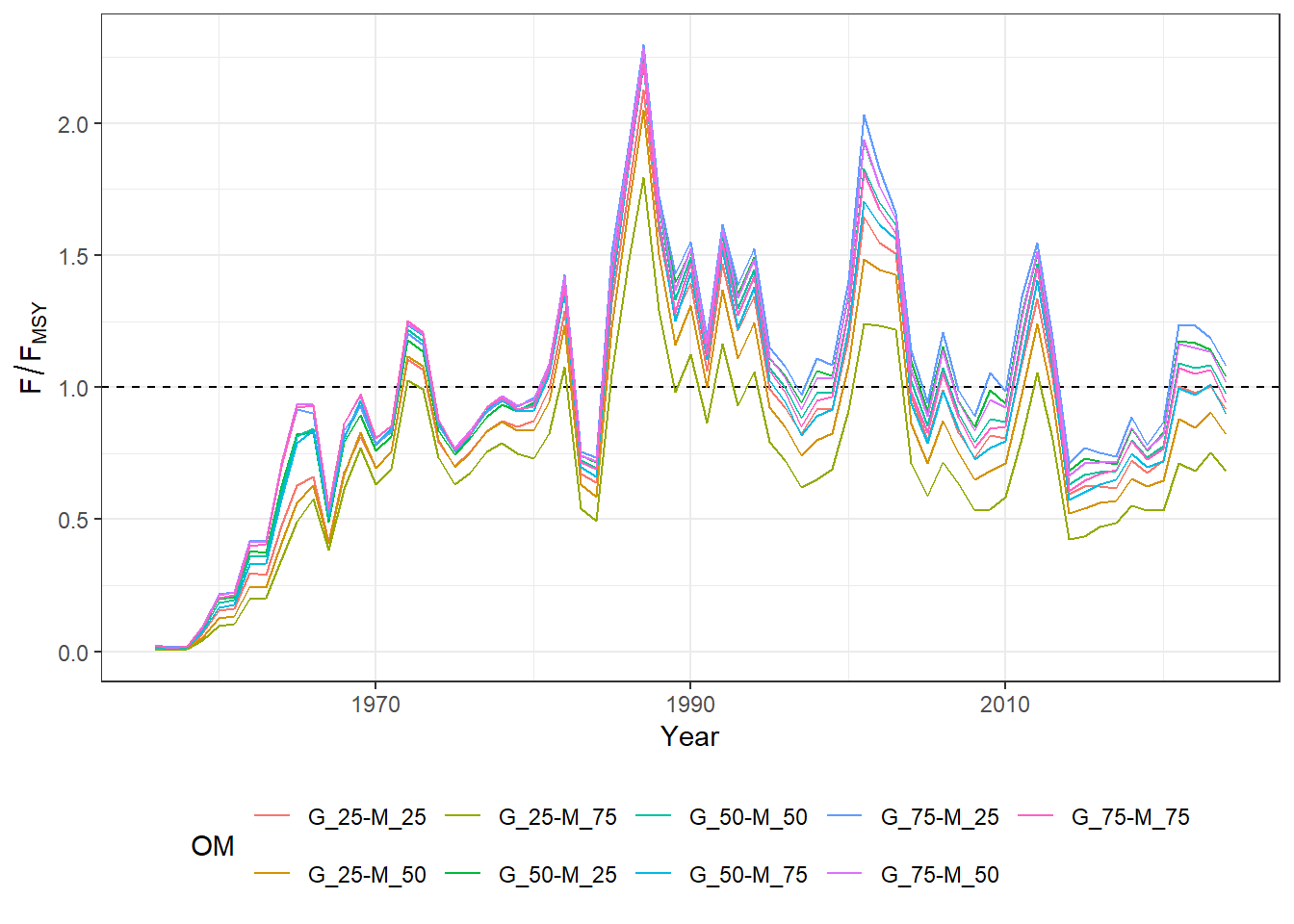
The figures below provide an overview of the population dynamics described in the nine Reference OMs:

Figure 3.2: historical spawning biomass
Figure 3.3: historical spawning biomass relative to equilibrium unfished level
Figure 3.4: historical spawning biomass relative to the MSY level
Figure 3.5: historical fishing mortality relative to the \(F_\text{MSY}\)

Table 3.3 summarises the MSY reference points, along with terminal year \(F/F_\text{MSY}\) and \(SB/SB_\text{MSY}\), for each of the nine Reference OMs.

Figure 3.2: Historical spawning biomass (\(SB\)), coloured by operating model and faceted by the axes of uncertainty

Figure 3.3: Historical spawning biomass depletion (\(SB/SB_0\)), by operating model.

Figure 3.4: Historical spawning biomass relative to MSY level (\(SB/SB_{\text{MSY}}\)), by operating model.

Figure 3.5: Historical fishing mortality relative to FMSY level (\(F/F_{\text{MSY}}\)), by operating model.

3.2 Reference Points

Table 3.3: MSY reference points and terminal year status, by operating model.

OM	F_MSY	SB_MSY	SPR_MSY	MSY	F/F_MSY	SB/SB_MSY
G_25-M_25	0.465	36506.59	0.284	24162.66	0.918	1.032
G_25-M_50	0.760	25046.72	0.275	24677.31	0.822	1.107
G_25-M_75	1.317	17418.31	0.266	25578.60	0.684	1.259
G_50-M_25	0.318	36215.84	0.278	23965.60	1.042	0.904
G_50-M_50	0.420	24274.44	0.270	24333.31	0.974	0.943
G_50-M_75	0.576	16222.00	0.262	24755.52	0.898	1.008
G_75-M_25	0.277	35422.99	0.275	23973.50	1.081	0.861
G_75-M_50	0.333	23292.29	0.267	24336.83	1.017	0.907
G_75-M_75	0.414	15219.33	0.259	24727.88	0.942	0.972